It is a measure of inequality developed by the Italian statistician Corrado Gini and published in 1912. It varies from 0 to 1, where 0 corresponds to complete equality and 1 corresponds to complete inequality. In this work the inequality of the distribution of calories among rabbits is calculated at the end of each time step.

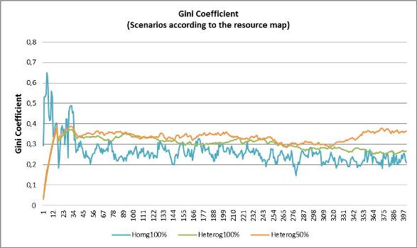
-Gini coefficient proved high in heterogeneous landscapes , demonstrating unequal resource consumption among agents. In homogeneous landscapes were found low coefficient values, demonstrating an equal consumption of resources between agents. Thus, it can be concluded that the distribution of resources, quantitative or through space, affects the value of the coefficient.

Gini Coefficient in three different landscapes: Hom 100- with resources distributed homogeneously, Het 100-with the same amount of resources distributed heterogeneously and Het 50-with half of resources amount distributed heterogeneously

-The agent population stabilizes regardless of the distribution of resources in the landscape and the amount of resources consumed by each agent according to the group to which it belongs.

Number of agents in three different landscapes: Hom 100- with resources distributed homogeneously, Het 100-with the same amount of resources distributed heterogeneously and Het 50-with half of resources amount distributed heterogeneously.
The graph shows that in the three scenarios there is a rapid growth in the first steps of the model followed by a decrease in amount of agents since the first 200 rabbits die almost at the same time because of the age. Then we can see the 3 populations stabilizing in different ways.

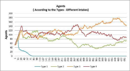
Number of agents, using Hetererogeneous 100 landscape map, divided by different Maximum absorption capacity of resources according to the groups which each agent belongs. In this case: Type 1 (17 calories), type 2 (19 calories), type 3 (22 calories) and type 4 (25 calories).
We can see that only type 1 group, that eats much less than it needs to survive in one step, had its population extinct by starvation, considering that it had exhalted its calorie stock to survive in few steps. Type 2 group also eats less than it needs to survive in one step and has to use its stock to survive. But the depletion of its stock was not enough to cause its death by starvation before “natural” death by age. The other two groups eat more than they need to survive and accumulate calories, but the model doesn't have any rule that favors rabbits with bigger stocks of calories in the birth process. So, the population dynamics of these types are random as model's processes are probabilistic.

-There are many more deaths by starvation in heterogeneous landsacapes and this number is bigger in scenarios with less amount of resources

In the three scerarios we can see a lot of deaths in the first steps of the model. That is because of the deaths of Type 1 rabbits which eat much less than they need to survive. After the first model steps there are no deaths by starvation in homogeneous scenario and most of the deaths occours in the heterogeneous scenario with half amount of resources. That happens because the rabbits that are born in areas with few resources units in heterogeneous lanscapes can't accumulate energy and use their stock util it reachs zero calories and die by starvation.

-The amount of resources available stabilizes as the population also stabilizes leading the amount of resources consumed to a dynamic equilibrium considering also that there is a resource recovery process in the model.

Movies were produced using rabbits position maps and landscape maps, outputs of the end of each step of the model considering three different scenarios

The black points are the agents moving across the landscape that is represented by diffrent colors according to the amount of resorcuces in each cell. Colors closed to red represents larger amount of resources, and colors closed to blue represents smaller amount of resources.

Homogeneous scenario: every cell has the same value in this map: 100 - average cell value: 100 -

Heterogeneous scenario: cells have different values in this map: 0 to 147 - average cell value: 100 -

Heterogeneous scenario: cells have different values in this map: 0 to 73 - average cell value: 50 -

In landscapes with heterogeneous distribution of resources, the agents move to the locations where are the greatest concentrations of resources. So, this areas are deprecated first and keep recovering their resources during model steps.

Back to Home

Next section

The study of population dynamics and movement of organisms that includes internal state, the ability to move and navigation of the agents, can provide insights about how individuals are affected by the characteristics of the matrix in which they are inserted (Nathan et al., 2008; McLane et al., 2011).

Through the results of this work it possible to see that spatially explicit modeling associated with agent based approach works as a good methodology to represent the environment of agents population and the dynamics of the interaction between individual and environment. It is also possible to highlight the causal relationships among movement, individual attributes and internal state, demographic and environmental changes. Thus, properties that improve the understanding of individual and demographic characteristics of spatially structured population can emerge from studies like this.