This is an old revision of the document!
Spatial Patterns of Changes
As Dinamica EGO was designed to be a general purpose dynamic modeling software, we present a collection of spatial patterns produced by the various combinations of its transition functions. In order to evaluate the wide range of Dinamias’s possibilities, a series of simulation were run using synthetic simplified maps. The results for each model are presented as follows:
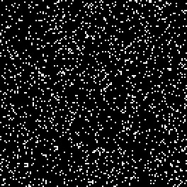
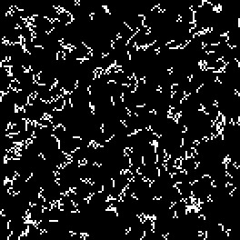
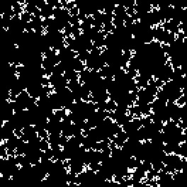
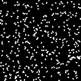
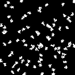
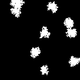
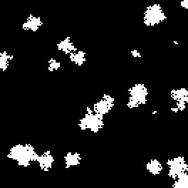
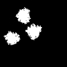
H0 to H8 are run, for a sole time step, by using a transition matrix 2×2 that models only one transition – from class 2 to 1 – with a rate of 0.01. The landscape map encompasses a matrix of 132 by 132 cells and all cells have equivalent spatial transition probability, which means that ancillary variables are not used to influence the cell allocation process.
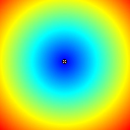
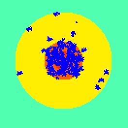
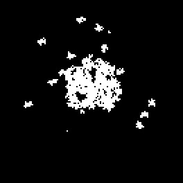
H9: Transitions occur as a function of the spatial probability. DINAMICA sets up a spatial transition probability map for each transition, based on the weights of evidence chosen for specific ranges of each spatial variable stored in the static cube raster dataset. Simulation is run in 15 steps, with a rate of 0.005 per step for transition 2-1. Only the Patcher function is used with patch mean size of 20 and patch variance of 0. Patch isometry is equal to 2. As a result, patches tend to form around the center of the map. The figures bellow depict, respectively, the static variable map, the calculated spatial transition probability map, and the simulated landscape.
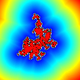
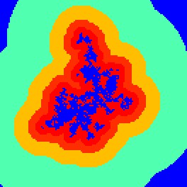
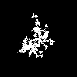
H10: Transitions occur as a function of dynamic spatial probability. DINAMICA calculates dynamic distances to cells in previous state 2 and uses it to set up a spatial transition probability map based on the weights of evidence chosen for specific ranges of distance. Since a dynamic distance map is used, a new transition map is calculated during each iteration. Simulation is run in 15 steps, with a rate of 0.005 per step for the transition 1 to 2. Only the Patcher function is used with patch mean size of 20 and patch variance of 0. Patch isometry is equal to 2. As a result, patches tend to nucleate around previous patches. The figures bellow depict, respectively, the dynamic distance map, the dynamically calculated spatial transition probability map, and the simulated landscape.
To test its a ability in simulating multiple transitions, simulations from H11 to H15 are run for a transition matrix 6 by 6. See figure bellow.
H11: There is no spatial arrangement and no patch aggregation. Expander percentage is 0, patch mean size is 1, and patch variance is 0. Transitions take place randomly only obeying the amounts of change set by the transition matrix. Simulations are run for 10 time steps. The figures bellow depict, respectively, the original landscape map, and the simulated landscape.
