To conduct our analysis we combine spatially explicit modeling, stakeholder engagement (semi-structured interviews and focus groups with selected agents in the rubber chain), and economic valuation.
The major rubber products (PVP, LSS, and LL) differ in terms of fixed production and operating costs and prices. Our model is prepared to compute different total costs for each product that include materials and time demanded for cleaning roads, collecting latex, internal transport (a map of land cover is used to spatially allocate the different means of transport), post-harvest treatments of latex, and storage.
Rubber model includes the following steps:
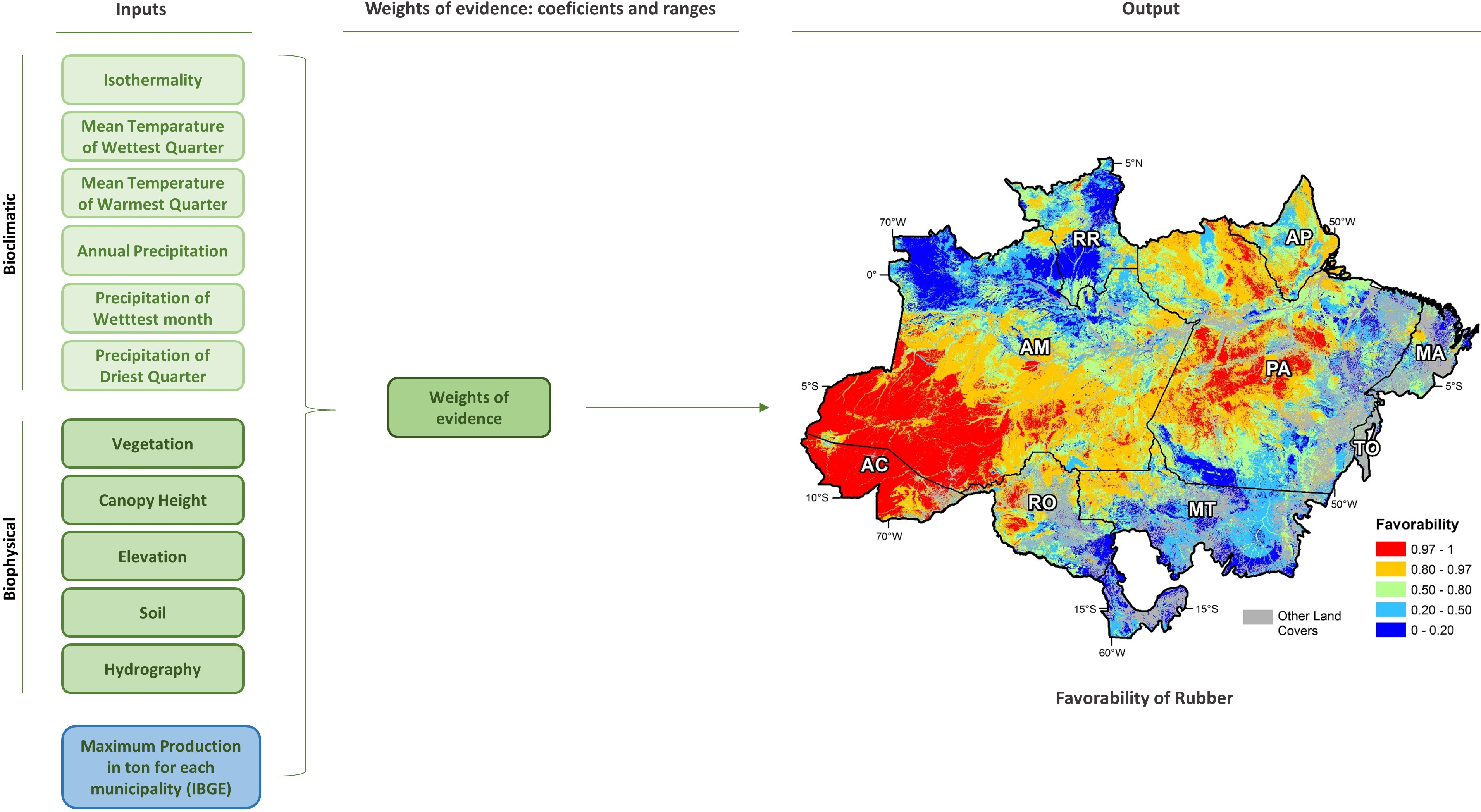
Using the method of Weights of Evidence (CITE) we integrated a set of biophysical and bioclimatic variables [3] as well as time-series (1994-2013) of production data from IBGE [4]. Production data were used as a surrogate for production capacity based on the assumption that a given jurisdiction (in this case Municipality) is still capable of producing the largest annual volume recorded over the past 20 years. The favorability map was transformed into rubber yields (kg/ha/year) based on the Probability Density Function (PDF) of rubber yields in the Acre case study [3]. We estimate that the potential annual rubber production in the Brazilian Amazon may be as high as 1.36 million tons.
The potential rents (US$/ha/year) are calculated according to the following equation:
Rent j = (Qxy*Pn)-(Qxy*CTprdn)-(Qxy*Ctrn*dz))
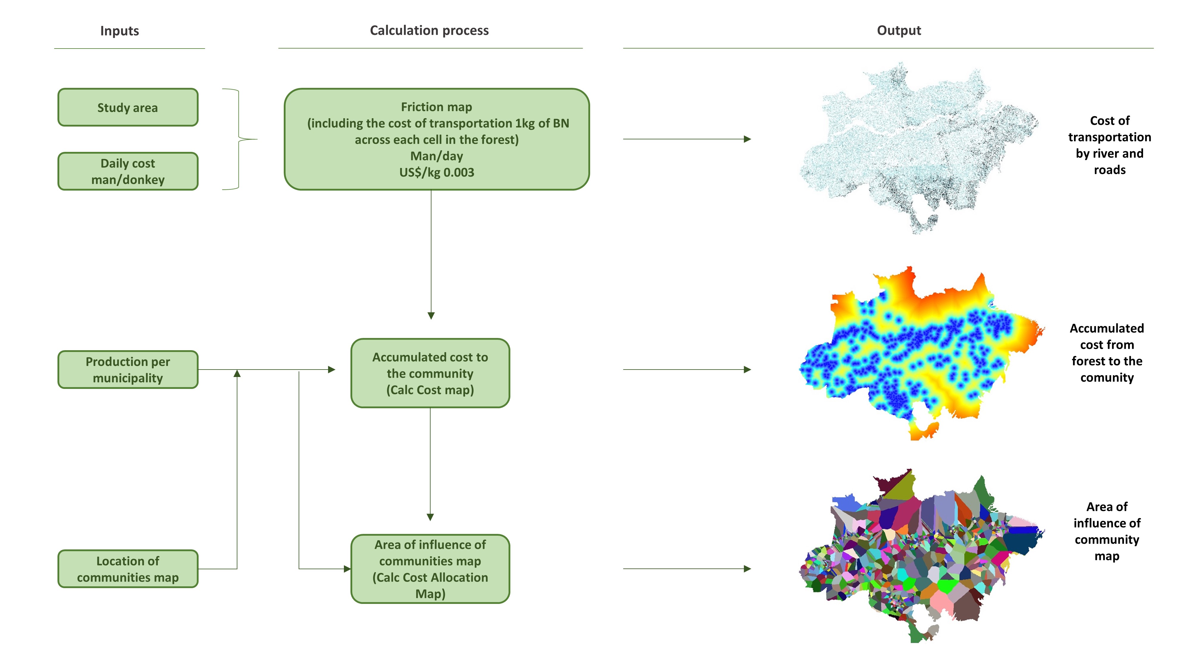
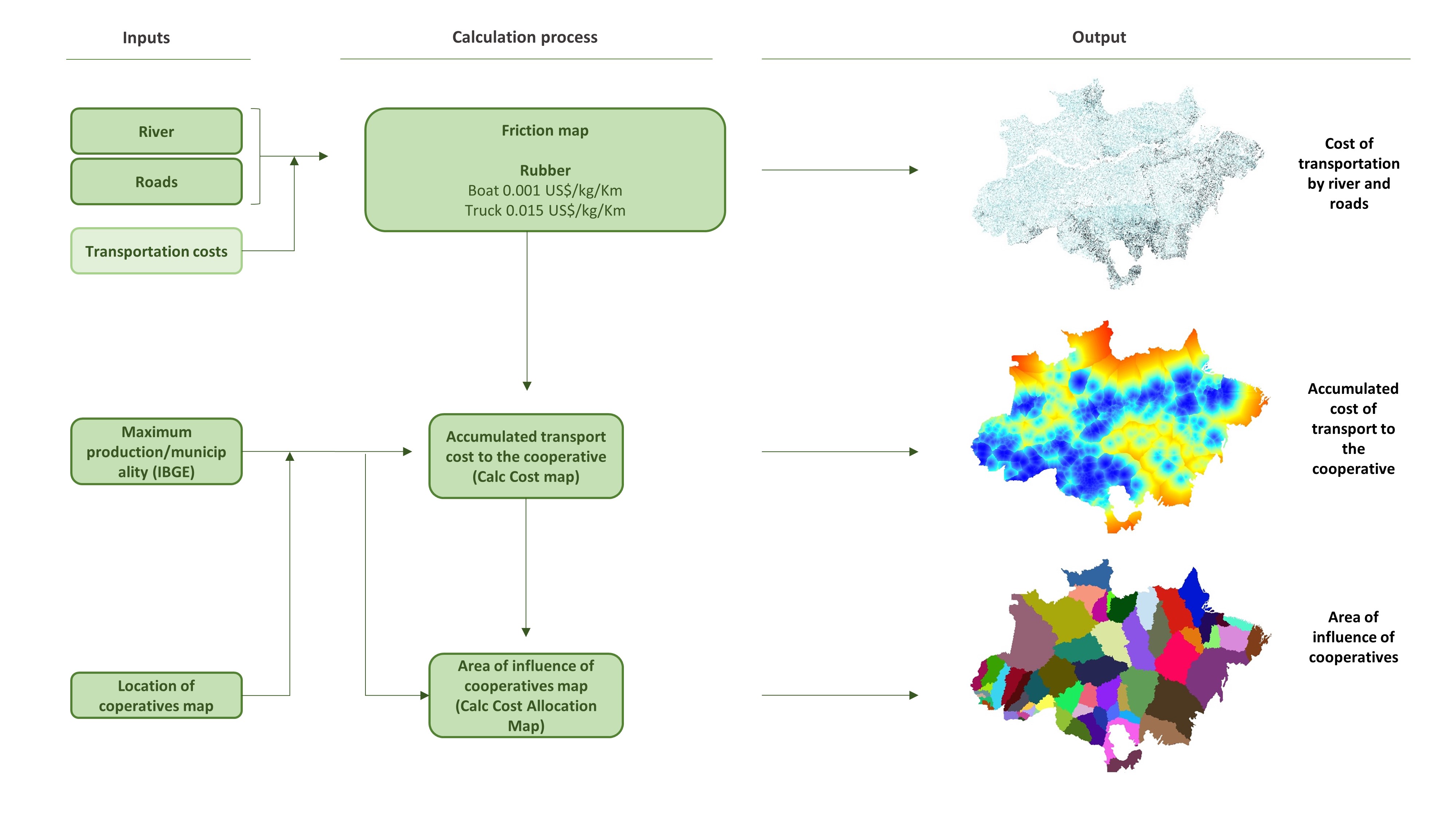
where Qxy is the simulated production for a cell with coordinates (x,y) in kg/ha; Pn and CTprdn correspond to respectively, selling price and the cost of production in US$/kg of product n and the cost of secondary transportation (Ctrn) of the product n by means (dz) from the location (x,y) to the nearest cooperative. We estimated transport costs for rubber across the forest and from the communities to the nearest cooperative. We then combined these maps into the accumulated transportation cost from the forest to the cooperative (see figures below).
1. SEAPROF – Secretaria Extensão Agroflorestal e Produção Familiar. Diagnóstico da cadeia de valor da borracha. 2014.
2. IBGE – Instituto Brasileiro de Geografia e Estatística. Produção da Extração Vegetal e da Silvicultura. 2015. Available from: www.ibge.gov.br/home/estatistica/economia/pevs/2013/default.sht.
3. Jaramillo, C.G. et al. Is It Possible to Make Rubber Extraction Ecologically and Economically Viable in the Amazon? The Southern Acre and Chico Mendes Reserve Case Study. Ecological Economics, 2017. 134: p. 186-197.
4. IBGE – Instituto Brasileiro de Geografia e Estatística. Produção da Extração Vegetal e da Silvicultura. 2015. Available from: https://www.ibge.gov.br/home/estatistica/economia/pevs/2013/default.shtm.
5. CONAB – Companhia Nacional de Abastecimento. Borracha natural, conjuntura mensal. 2014.
Download report