Using Sojourn Time
Load the model simulate_deforestation_and_abandonment_using_sojourn_time.egoml from \Guidebook_Dinamica_5\Models\additional_resources_lucc\sojourn_time\simulate_deforestation_and_abandonment_using_sojourn_time.
The use of sojourn time implies that a specific transition or event will not occur unless a certain time has passed since a specific event has occurred.
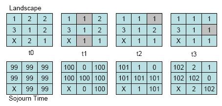
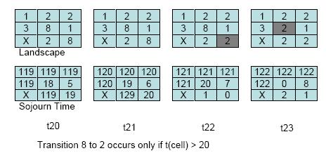
The concept of sojourn time can be implemented using a map that keeps track of the time since a particular event has occurred (for example, a transition from state i to j). For each cell, a clock will count the time past after a particular event has occurred. In the end of iteration, this map is updated, if there is no new event, the model simply adds one to the cell’s sojourn time, and if an event occurs, the clock is set to zero (Fig.1).
The sojourn time can be used as a rule to constrain a transition from a state to the other only after a certain sojourn in a particular state. In this example, the sojourn time is used to influence the probabilities from deforested land (value 1) to abandon – regrowth (value 8). Land is only abandoned after 4 years in use: i.e. after deforestation has taken place (transition 2 to 1).
The sojourn map is initialized with high values (e.g. 9999). By doing so, it’s possible to differentiate cells where a certain transition has never occurred from cells that have changed during the simulation. This might be useful for further analyses.
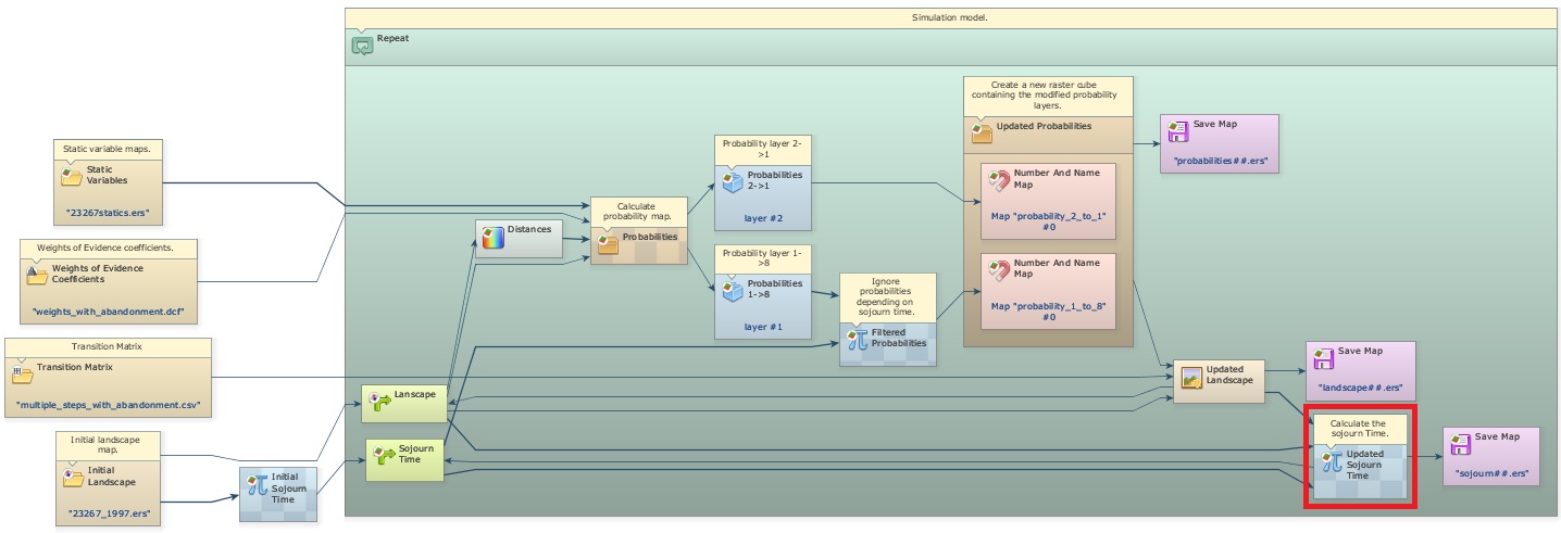
At the end of iteration, a new sojourn map is calculated by comparing the previous land-use map with the current one. Cells whose states have changed, the corresponding sojourn times are set to zero; otherwise they are incremented by one time unit.
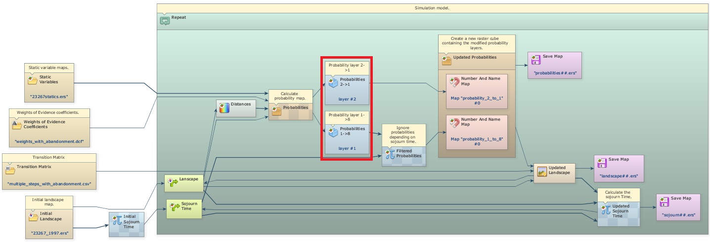
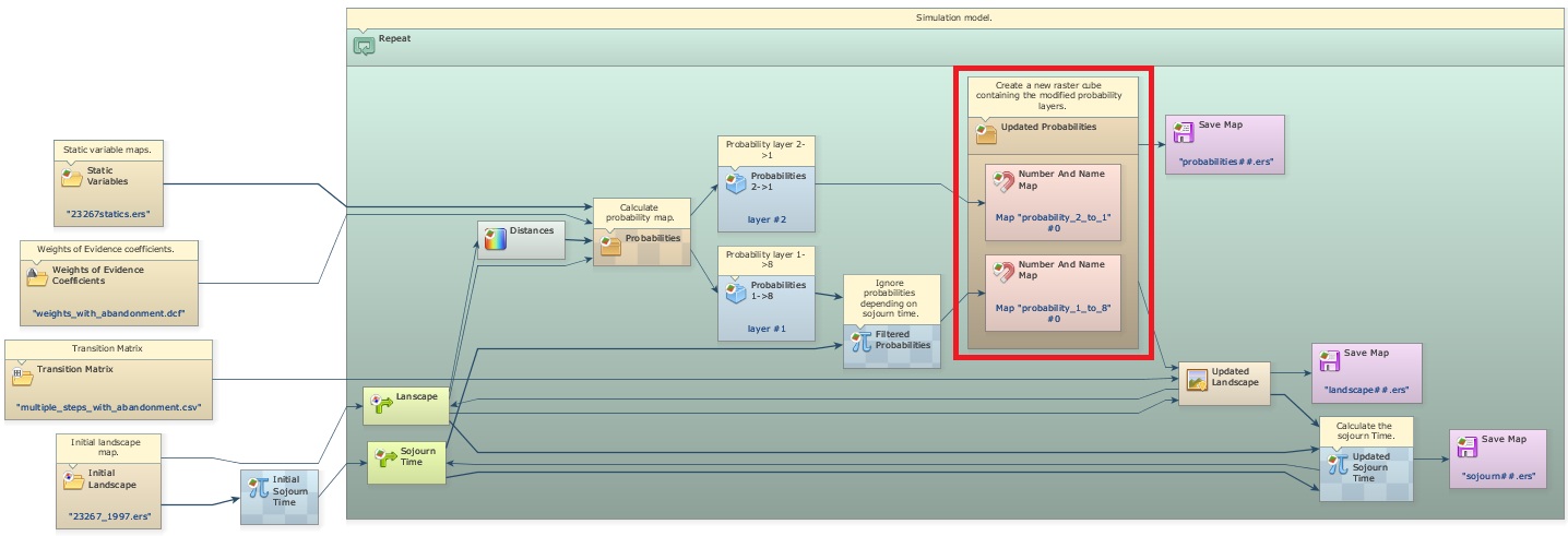
The sojourn time concept is applied to constrain a change. An easy way to do this is by modifying the corresponding probability map. As these maps are stacked in a cube raster set, you need first to extract the layers from the cube raster set, so the Calculate Map will be able to manipulate them separately.
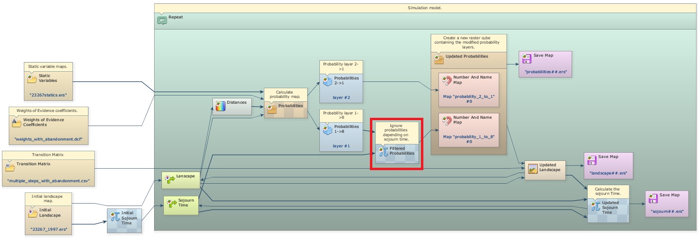
After calculating the probability map using Calc W. of E. Probability Map, the layer of the transition from deforested to abandon (transition 1 to 8) undergoes a new calculation. This is a comparison of the sojourn time. If a deforested cell is older than 3 years, its probability is kept unchanged. If it is not, the probability to change to abandon is set to zero, impeding, as result, this transition to take place.
Then, the probability layers (the original layer with transition 2 to 1 and the new layer with transition 1 to 8) are put together again as a new cube raster dataset, which is passed on to the transition functions, Expander and Patcher.
Using sojourn time and deterministic transitions
Load the model simulate_def_aband_and_deterministic_transition.egoml from \Guidebook_Dinamica_5\Models\additional_resources_lucc\sojourn_time\simulate_deforestation_and_abandonment_using_sojourn_time_and_deterministic_transition
In this example, transition from abandon (land abandoned undergoes regeneration) to forest is deterministically determined based only on the sojourn time. So after a period in regrowth, the abandoned parcel has acquired a forest structure similar to a mature forest, thereby considered as forest. The minimum sojourn time for this transition to occur is 21 years (Fig.2)
An additional transition from deforested land to abandon is added to the previous model. Calculate Categorical Map placed at the end of the model is employed to perform this transition. Its rule is the following:
if i1 = 8 and i2 > 20 then 2 else i1
i1 is the landscape map and i2 is the sojourn map (forest is 2, abandon is 8). Note that for simplicity, it’s not possible to clear areas in abandon (transition 8 to 1). This could be added to the model as a new transition. Texeira et al. (2009) provide an example of modeling the landscape dynamics of the Atlantic forest, which includes multistate and transition from forest to various land-use.
